I regularly use the system-level activity chart available in Enterprise Manager. In my opinion it is a simple and effective way to know how much a specific database is loaded at a specific time. This is for example an interesting way for observing how a specific load is processed (see this post for an example).
Unfortunately it also happens that this possibility is not available. The main reasons I faced in the past are the following:
- Standard Edition is used
- Enterprise Edition is used but Diagnostic Pack is not licensed
- Enterprise Manager is not available
- GUI is not available
The aim of this post is to present you a utility that I wrote to cope with these restrictions. It goes without saying that its main purpose is to display information similar to the one provided by the system-level activity chart when working in Standard Edition (or Enterprise without Diagnostic Pack) in a terminal. And that, with both 10g and 11g.
Several dynamic performance views externalize information that can be used for displaying the activity of a system. The two I chose are v$sys_time_model and v$system_wait_class. The challenge of using these views is that they provide only cumulative statistics that are incremented on a regular basis. It is therefore necessary to use a utility that samples the information they provide. In other words, to find out how much a specific statistic changes over a short period of time.
The utility is based on three scripts:
- system_activity_setup.sql: install the objects required by the system_activity.sql script
- system_activity.sql: show the database activity at system level
- system_activity_teardown.sql: remove the objects required by the system_activity.sql script
To install the utility execute, as SYS, the system_activity_setup.sql script. It creates several object types, a function (the core of the utility) and a public synonym. In addition it grants the privilege to execute the function to public.
To use the utility you can directly call the system_activity function or, to have a decent output, execute the system_activity.sql script in SQL*Plus. As the following example shows the script requires two parameters:
- The first parameter, interval, specifies in seconds how much time to wait to compute the deltas. Since the database engine does not update the statistics in real-time, specifying less than 10-15 seconds is usually pointless.
- The second parameter, count, specifies the number of samples.
SQL> @system_activity 15 50

                                       DBS112.ANTOGNINI.CH / 2011-02-28

Time     AvgActSess Other% Queue%   Net%   Adm%  Conf%  Comm%  Appl%  Conc% Clust% SysIO% UsrIO% Sched%   CPU%
-------- ---------- ------ ------ ------ ------ ------ ------ ------ ------ ------ ------ ------ ------ ------
06:30:19        1.1    0.0    0.0    0.0    0.0    0.0    0.8    0.0    0.0    0.0    1.6   89.9    0.0    7.7
06:30:34        1.5    0.0    0.0    0.0    0.0    0.0    0.9    0.0    0.3    0.0    2.2   87.5    0.0    9.2
06:30:49        1.2    0.0    0.0    0.1    0.0    0.0    0.7    0.0    0.0    0.0    1.4   91.3    0.0    6.5
06:31:04        1.2    0.7    0.0    0.0    0.0    0.0    0.8    0.0    0.0    0.0    1.7   89.6    0.0    7.3
06:31:19        1.1    0.0    0.0    0.0    0.0    0.0    0.8    0.0    0.0    0.0    1.6   86.1    0.0   11.5
06:31:34        1.4    0.0    0.0    0.0    0.0    0.0    0.6    0.0    0.2    0.0    1.3   91.8    0.0    6.0
06:31:49        1.0    0.0    0.0    0.0    0.0    0.0    0.8    0.0    0.0    0.0    1.7   89.6    0.0    7.9
06:32:04        1.1    0.0    0.0    0.0    0.0    0.0    0.7    0.0    0.0    0.0    1.6   90.2    0.0    7.5
06:32:19        1.1    0.0    0.0    0.1    0.0    0.0    0.8    0.0    0.0    0.0    1.7   89.1    0.0    8.4
06:32:34        1.1    0.1    0.0    0.0    0.0    0.0    0.7    0.0    0.2    0.0    1.7   89.9    0.0    7.4
06:32:49        1.0    0.0    0.0    0.0    0.0    0.0    0.6    0.0    0.0    0.0    1.7   90.3    0.0    7.3
06:33:04        1.1    0.0    0.0    0.0    0.0    0.0    0.7    0.0    0.0    0.0    1.7   90.5    0.0    7.0
06:33:19        1.1    0.0    0.0    0.0    0.0    0.0    1.2    0.0    0.0    0.0    1.9   89.4    0.0    7.4
06:33:34        1.1    0.0    0.0    0.1    0.0    0.1    0.7    0.0    0.2    0.0    1.8   88.8    0.0    8.4
06:33:49        1.3   17.3    0.0    0.0    0.0    0.0    0.6    0.0    0.0    0.0    1.5   74.7    0.0    5.9
06:34:04        1.4   22.6    0.0    0.0    0.0    0.0    0.6    0.0    0.0    0.0    1.2   69.3    0.0    6.3
06:34:19        1.1    0.0    0.0    0.0    0.0    0.0    0.8    0.0    0.0    0.0    1.7   89.6    0.0    8.0
06:34:34        1.0    0.0    0.0    0.0    0.0    0.0    0.7    0.0    0.2    0.0    2.2   89.3    0.0    7.7
06:34:49        1.1    0.1    0.0    0.0    0.0    0.0    0.6    0.0    0.0    0.0    1.4   91.0    0.0    6.9
06:35:04        1.2   -0.1    0.0    0.1    0.0    0.0    0.8    0.0    0.4    0.0    1.7   85.5    0.0   11.6
06:35:19        6.0    0.0    0.0    0.0    0.0    0.0    1.0    0.0    0.0    0.0    1.7   88.8    0.0    8.5
06:35:34        7.4    0.0    0.0    0.0    0.0    0.0    0.8    0.0    0.0    0.0    1.9   91.2    0.0    6.0
06:35:49        7.1    0.0    0.0    0.0    0.0    0.5    1.2    0.0    0.0    0.0    1.9   90.7    0.0    5.7
06:36:04        7.2    0.9    0.0    0.0    0.0    0.0    0.9    0.0    0.0    0.0    1.7   90.7    0.0    5.8
06:36:19        7.2    0.0    0.0    0.0    0.0    0.0    1.0    0.0    0.0    0.0    1.8   90.9    0.0    6.3
06:36:34        6.8    0.0    0.0    0.0    0.0    0.0    1.0    0.0    0.0    0.0    1.7   91.3    0.0    6.0
06:36:49        7.1    0.0    0.0    0.0    0.0    0.5    1.1    0.0    0.0    0.0    1.9   90.9    0.0    5.6
06:37:04        6.9    0.0    0.0    0.0    0.0    0.0    1.0    0.0    0.0    0.0    1.8   91.3    0.0    5.9
06:37:19        6.9    0.0    0.0    0.0    0.0    0.0    0.9    0.0    0.0    0.0    1.7   91.7    0.0    5.7
06:37:34        7.1    0.0    0.0    0.0    0.0    0.0    0.9    0.0    0.0    0.0    1.8   91.6    0.0    5.8
06:37:49        6.9    0.0    0.0    0.0    0.0    0.0    1.1    0.0    0.0    0.0    1.8   91.3    0.0    5.8
06:38:04        7.0    0.0    0.0    0.0    0.0    1.1    1.0    0.0    0.2    0.0    1.9   90.2    0.0    5.7
06:38:19        6.8    0.0    0.0    0.0    0.0    0.0    0.9    0.0    0.0    0.0    1.6   91.6    0.0    5.9
06:38:34        7.2    0.3    0.0    0.0    0.0    0.0    0.9    0.0    0.0    0.0    1.7   91.0    0.0    6.0
06:38:49        6.7    0.0    0.0    0.0    0.0    0.0    1.1    0.0    0.0    0.0    1.7   91.4    0.0    5.8
06:39:04        7.4    0.0    0.0    0.0    0.0    0.4    1.2    0.0    0.0    0.0    2.0   90.9    0.0    5.5
06:39:19        2.0   -0.3    0.0    0.0    0.0    0.0    1.6    0.0    0.1    0.0    2.0   86.5    0.0   10.1
06:39:34        1.1    0.0    0.0    0.1    0.0    0.0    0.7    0.0    0.2    0.0    1.7   89.2    0.0    8.1
06:39:49        1.1    0.0    0.0    0.0    0.0    0.0    0.9    0.0    0.0    0.0    1.8   89.6    0.0    7.6
06:40:04        1.1    0.0    0.0    0.0    0.0    0.0    0.8    0.0    0.0    0.0    2.1   89.6    0.0    7.6
06:40:19        1.5   14.4    0.0    0.0    0.0    0.0    0.7    0.0    1.1    0.0    1.3   74.3    0.0    8.3
06:40:34        1.6   -0.2    0.0    0.0    0.0    0.0    0.6    0.0    0.3    0.0    1.4   87.7    0.0   10.2
06:40:49        1.3    0.0    0.0    0.1    0.0    0.0    0.6    0.0    0.0    0.0    1.6   91.2    0.0    6.5
06:41:04        1.2    0.9    0.0    0.0    0.0    0.0    0.7    0.0    0.0    0.0    1.7   89.5    0.0    7.3
06:41:19        1.2    0.0    0.0    0.0    0.0    0.0    0.7    0.0    0.0    0.0    1.8   87.3    0.0   10.3
06:41:34        1.3    0.0    0.0    0.0    0.0    0.0    0.5    0.0    0.1    0.0    1.4   91.5    0.0    6.3
06:41:49        1.1    0.1    0.0    0.0    0.0    0.0    0.8    0.0    0.0    0.0    1.6   90.3    0.0    7.2
06:42:04        1.1    0.0    0.0    0.1    0.0    0.0    0.8    0.0    0.0    0.0    2.0   89.9    0.0    7.2
06:42:19        1.1    0.0    0.0    0.0    0.0    0.0    0.7    0.0    0.0    0.0    1.5   90.8    0.0    7.1
06:42:34        1.1    0.0    0.0    0.0    0.0    0.0    0.8    0.0    0.2    0.0    2.0   89.4    0.0    7.6
The output provides:
- the timestamp of the end of the sampling period,
- the number of average active sessions, and
- the percentage of time spent for each wait class and CPU.
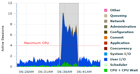
For comparison purposes, here is the activity chart for the very same period of time. Even though the data is not exactly the same (the activity chart is based on ASH, a completely different source of information), it is good enough to know how much a database is loaded and which wait class is the major contributor.
Any feedback or suggestion to improve the scripts is highly welcome.
Don’t forget Ash Viewer (http://sourceforge.net/projects/ashv/).
You can run it in standard mode and it doesn’t use the ASH views, so you can use it without D&T pack, or on older database versions.
Cheers
Tim…
Hi Tim
I do not forget it… but, AFAIK, it doesn’t fulfill the “No GUI” requirement.
Cheers,
Chris
Sorry to say but v$active_session_history is a part of the Oracle Diagnostic Pack and requires additional license.
Hi
Of course you are right. But, honestly, since in this post I’m not using/referring to v$active_session_history, I don’t understand why you are pointing it out.
Best,
Chris
Very nice!
This could also be included in some DB monitoring or even RRD tool in front of this.
Hi Christian,
Nice scripts. The continuous output with pipeline is cool. I first saw this with Adrian and Tanel’s moats.sql. Definitely something I want to play around with more. I modified moats.sql to show average I/O latency and histogram for the I/O events and sent it off to Adrian to see if he wanted to include it. In the mean time I have been meaning to pull this I/O part out into it’s own script so I could blog about it. Given your nice example, that may make the job easier.
The ashviewer is cool as well.
For web enabled ( fails the “no gui” test, though output could be converted to ascii :P ) I put together a highcharts (jquery library) interface that is pretty much like the top activity page with area selection and drilldown and it works without the diagnostics pack: http://dboptimizer.com/2011/10/31/w-ash-web-enabled-ash/
It was mainly a proof of concept. Should probably put it on github and start iterating and improving it.
– Kyle Hailey
Hello:
I do agree completely with the “No GUI” requirement, but sometimes a picture is worth a thousand words.
Depending on who you are discussing your data with, or to better understand correlations among values, I found GnuPlot being an invaluable too.
So I propose to integrate the script with an optional step to plot the data.
Supposing that the performance data goes spooled on a file named “gpash.txt”, the parameter file could be like this (save with name, say, “gpash.gp”):
# Gnuplot script for ASH style graphs

set terminal jpeg font "./LiberationMono-Regular.ttf,10" noenhanced size 768,384

set output "gpash.jpg"

set autoscale

set decimalsign locale "en_US.UTF8"  # on Windows use "american"

set title "Top Activity"

set ylabel "Active Sessions"

set grid xtics ytics

set xdata time

set format x "%H:%M:%S"

set timefmt "%H:%M:%S"

set style line   3 linecolor rgbcolor "#F06EAA" # pink             Other

set style line  11 linecolor rgbcolor "#C9C2AF" # lightest-brown   Cluster

set style line   4 linecolor rgbcolor "#C2B79B" # lighter-brown    Queuing

set style line   5 linecolor rgbcolor "#9F9371" # light-brown      Network

set style line   6 linecolor rgbcolor "#717354" # med-brown        Administrative

set style line   7 linecolor rgbcolor "#5C440B" # dark-brown       Configuration

set style line   8 linecolor rgbcolor "#E46800" # orange           Commit

set style line   9 linecolor rgbcolor "#C02800" # red              Application

set style line  10 linecolor rgbcolor "#8B1A00" # brick            Concurrency

set style line  12 linecolor rgbcolor "#0094E7" # light-blue       System I/O

set style line  13 linecolor rgbcolor "#004AE7" # dark-blue        User I/O

set style line  14 linecolor rgbcolor "#CCFFCC" # light-green      Scheduler

set style line  15 linecolor rgbcolor "#00CC00" # green            CPU

set style data lines

plot

"gpash.txt" every ::2 using 1:($2*($3+$4+$5+$6+$7+$8+$9+$10+$11+$12+$13+$14+$15)/100) linestyle 3 title "Other" with filledcurve x1,

"" every ::2 using 1:($2*($4+$5+$6+$7+$8+$9+$10+$11+$12+$13+$14+$15)/100) linestyle 11 title "Cluster" with filledcurve x1,

"" every ::2 using 1:($2*($4+$5+$6+$7+$8+$9+$10+$12+$13+$14+$15)/100) linestyle 4 title "Queueing" with filledcurve x1,

"" every ::2 using 1:($2*($5+$6+$7+$8+$9+$10+$12+$13+$14+$15)/100) linestyle 5 title "Network" with filledcurve x1,

"" every ::2 using 1:($2*($6+$7+$8+$9+$10+$12+$13+$14+$15)/100) linestyle 6 title "Administrative" with filledcurve x1,

"" every ::2 using 1:($2*($7+$8+$9+$10+$12+$13+$14+$15)/100) linestyle 7 title "Configuration" with filledcurve x1,

"" every ::2 using 1:($2*($8+$9+$10+$12+$13+$14+$15)/100) linestyle 8 title "Commit" with filledcurve x1,

"" every ::2 using 1:($2*($9+$10+$12+$13+$14+$15)/100) linestyle 9 title "Application" with filledcurve x1,

"" every ::2 using 1:($2*($10+$12+$13+$14+$15)/100) linestyle 10 title "Concurrency" with filledcurve x1,

"" every ::2 using 1:($2*($12+$13+$14+$15)/100) linestyle 12 title "System I/O" with filledcurve x1,

"" every ::2 using 1:($2*($13+$14+$15)/100) linestyle 13 title "User I/O" with filledcurve x1,

"" every ::2 using 1:($2*($14+$15)/100) linestyle 14 title "Scheduler" with filledcurve x1,

"" every ::2 using 1:($2*($15)/100) linestyle 15 title "CPU" with filledcurve x1
Then you run with the command “gnuplot gpash.gp”.
You can see the resulting image here.
Hope you like it,
Andrea
Hi Andrea
Thank you very much for the nice example. I personally like Excel for this kind of stuff, though.
Cheers,
Chris
Hi Christian,
Really like the script and the blog.
Here is another sqlplus monitoring script…
http://thomasdale.wordpress.com/2012/06/13/whats-going-on-in-my-database/
Tom
I took the liberty to rewrite your script to skip the need for upfront object creation. Apart from that the only other difference is that the output is not printed live but at the end of the run.
Hi Christian,
today I’ve found your post and I’m very happy to find something for a Oracle Standard One Edition :)
I run the setup.sql and try the whole thing. It works great but I’m not sure that there are correct values. The value of CPU% says the most time 100% (or above 80%) but when I look at the comman top on the machine its’s only uses under 10% . So I looked into the setup script and there are coloums with l_cpu2 and l_cpu1. Have I to adapt the script for more available cpus?
Cheers,
Jessica
Hi Jessica
Be careful…
AvgActSess tells you how busy is the system (average number of active sessions).
All “%” values tells you how much DB Time is spent in each wait class. In other words, the sum of all “%” is always 100%.
An example:
– AvgActSess = 10
– CPU% = 80%
–> 10 * 0.8 = 8 CPUs are fully used
Best,
Chris
Hi Chris,
first of all: big thanks because of your fast answer an your good explanation!
Now it is much more easier for me to understand the whole thing :)
Cheers,
Jessica
First of all, thanks for sharing this!
I noticed that sometimes it prints negative number of active sessions. Anyone know why this happens?
Ex:
Hi
when you say “sometimes”, does that mean that for most of the time the values are good and, suddenly, wrong data is shown.
Best,
Chris
Hi Chris! Thanks for your reply.
Yes, for most of time the values are good. I were just trying to figure out why this was happening.
Thanks!